Introduction
This is a writeup for final project of the course Machine Learning, Fall 2024, originally intended as a machine learning competition, however, a data leakage was discovered, making it having an interesting solution to share. Credits to the professor and TAs for the wonderful course and final project.
Leaderboard placement
The final result of my solution ranks 7th in both stage 1 and stage 2 for both public and private scores.
| stage 1 public score | stage 1 private score | stage 2 public score | stage 2 private score |
|---|---|---|---|
| 0.94092 | 0.93262 | 0.86129 | 0.87336 |
Stage 1 public score
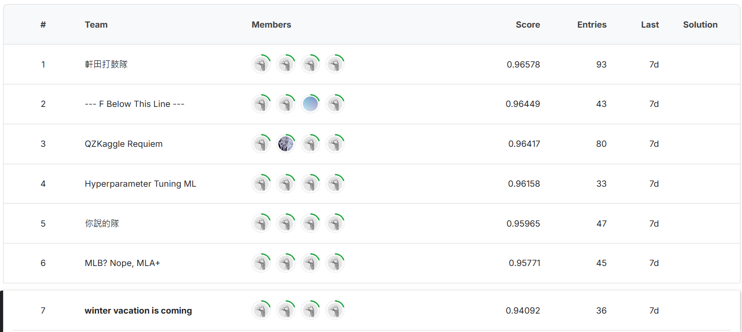
Stage 1 private score
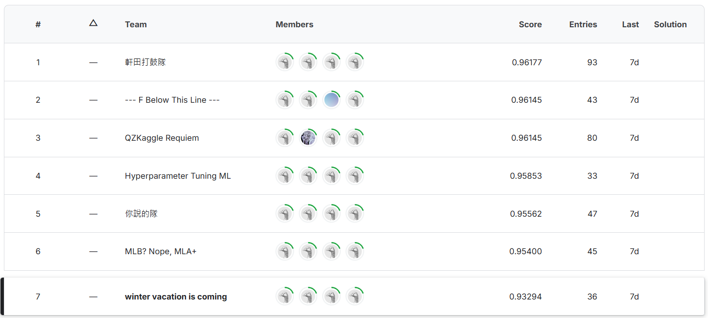
Stage 2 public score
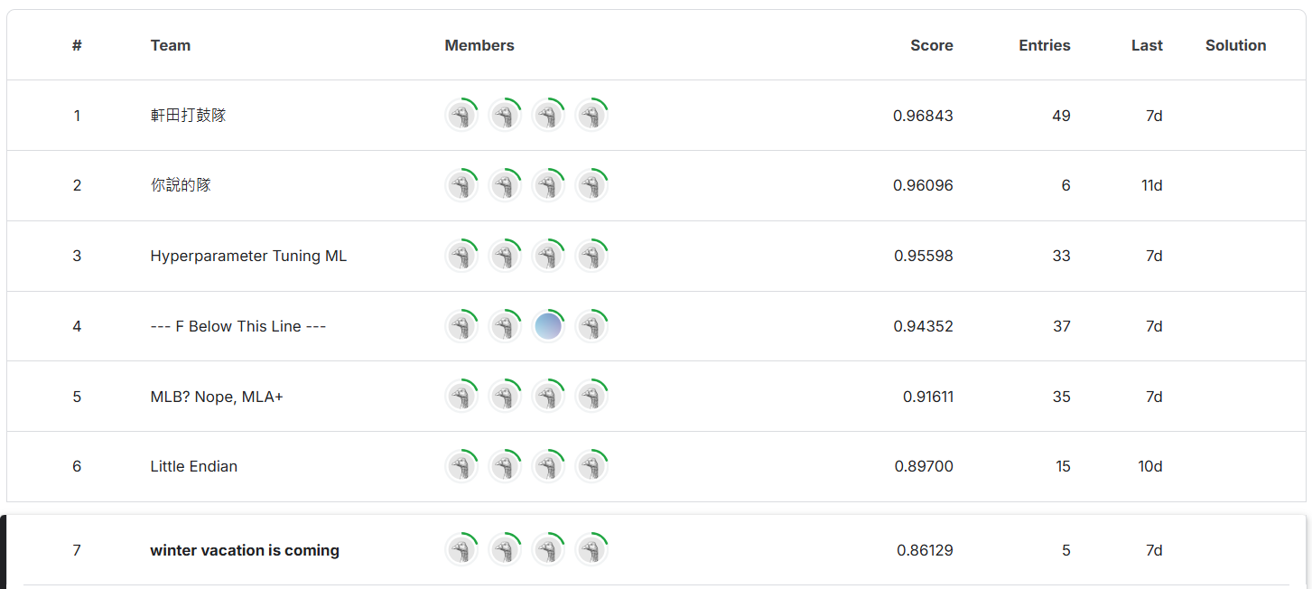
Stage 2 private score
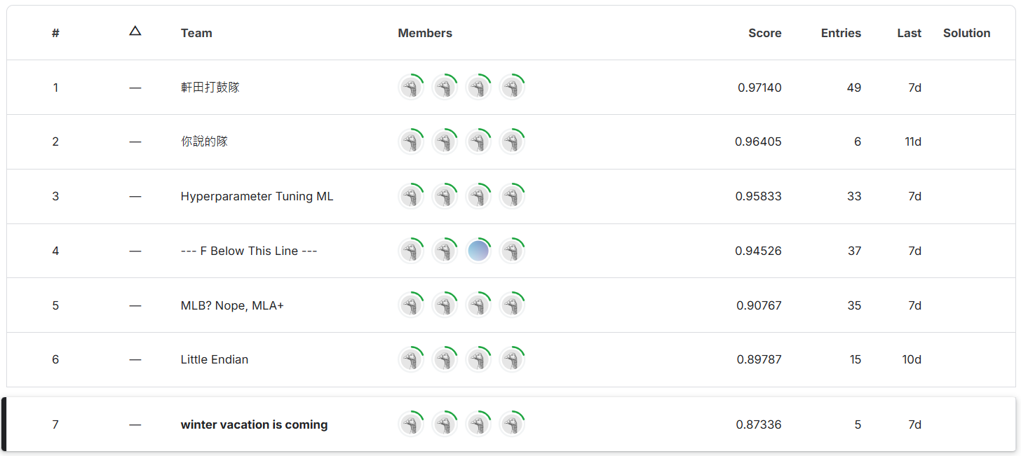
Motivation
After seeing there already exist a solution that can predict up to 96% accuracy, I immediately know it must be caused by data leakage, more specifically, feature (home_team_win) leakage. After asking ChatGPT for the possible feature, home_team_wins seem to be a important feature since it contains the result of each games.

Data Analysis
From the distribution of data it is clear that each column of the training data and testing data have been standardize across the whole dataset, how to retrieve the real (before standardize) value becomes the first problem.
Mean and Standard Deviation
First I guess that for team_wins data, each previous game(\(x\)) is represented by 1 if won, 0 if lose, therefore
Hence the range of team_wins_mean is \([0, 1]\) and the range of team_wins_std is \([0, \frac{1}{2}]\). Then apply the following formula to inverse the standardization
Last, sorts all the training data by date and calculate the count of wins to verify the value gets from the previous formula is almost always correct. Which can be verify with the following script. Note different values between team_wins and real_team_wins is caused by noises in the label (confirmed by the professor).
import numpy as np
import pandas as pd

train_data = pd.read_csv("train_data.csv", index_col = "id").sort_values("date")

train_data['home_team_wins_mean'] -= train_data['home_team_wins_mean'].min()
train_data['home_team_wins_mean'] /= train_data['home_team_wins_mean'].max()
train_data['away_team_wins_mean'] -= train_data['away_team_wins_mean'].min()
train_data['away_team_wins_mean'] /= train_data['away_team_wins_mean'].max()
train_data['home_team_wins_std'] -= train_data['home_team_wins_std'].min()
train_data['home_team_wins_std'] /= 2 * train_data['home_team_wins_std'].max()
train_data['away_team_wins_std'] -= train_data['away_team_wins_std'].min()
train_data['away_team_wins_std'] /= 2 * train_data['away_team_wins_std'].max()

data_2016_KFH = train_data.query("(home_team_abbr == 'KFH' or away_team_abbr == 'KFH') and season == 2016")
games = []
team_wins_mean = []
team_wins_std = []
real_team_wins_mean = []
real_team_wins_std = []
for index, row in data_2016_KFH.iterrows():
    real_team_wins_mean.append(np.array(games).mean())
    real_team_wins_std.append(np.array(games).std())
    if (row['home_team_abbr'] == 'KFH'):
        team_wins_mean.append(row['home_team_wins_mean'])
        team_wins_std.append(row['home_team_wins_std'])
    else:
        team_wins_mean.append(row['away_team_wins_mean'])
        team_wins_std.append(row['away_team_wins_std'])
    if (row['home_team_abbr'] == 'KFH') ^ row['home_team_win']:
        games.append(0)
    else:
        games.append(1)
data_2016_KFH['team_wins_mean'] = team_wins_mean
data_2016_KFH['team_wins_std'] = team_wins_std
data_2016_KFH['real_team_wins_mean'] = real_team_wins_mean
data_2016_KFH['real_team_wins_std'] = real_team_wins_std
print(data_2016_KFH[['date', 'team_wins_mean', 'real_team_wins_mean', 'team_wins_std', 'real_team_wins_std']].head(20))
             date  team_wins_mean  real_team_wins_mean  team_wins_std  real_team_wins_std
id
707    2016-04-03             NaN                  NaN            NaN                 NaN
9689   2016-04-04        0.000000             0.000000       0.000000            0.000000
8329   2016-04-05        0.000000             0.000000       0.000000            0.000000
6782   2016-04-06        0.333333             0.333333            NaN            0.471405
7122   2016-04-08        0.500000             0.500000       0.500000            0.500000
3364   2016-04-10        0.400000             0.400000       0.489898            0.489898
4949   2016-04-12        0.333333             0.333333       0.471405            0.471405
5528   2016-04-13        0.428571             0.428571       0.494872            0.494872
1539   2016-04-14        0.375000             0.375000       0.484123            0.484123
10049  2016-04-15        0.333333             0.333333       0.471405            0.471405
4231   2016-04-16        0.300000             0.300000            NaN            0.458258
5845   2016-04-17        0.363636             0.363636       0.481046            0.481046
6937   2016-04-19             NaN             0.416667       0.493007            0.493007
3765   2016-04-20        0.461538             0.461538       0.498519            0.498519
5418   2016-04-21             NaN             0.428571       0.494872            0.494872
8328   2016-04-22        0.466667             0.466667       0.498888            0.498888
7138   2016-04-23        0.437500             0.437500       0.496078            0.496078
9104   2016-04-24        0.411765             0.411765       0.492153            0.492153
3558   2016-04-25        0.444444             0.444444       0.496904            0.496904
5624   2016-04-26        0.473684             0.473684       0.499307            0.499307
Skewness
Next to get the inverse formula of team_wins_skew, first calculate the real skewness from the count of wins in the same way as verifying team_wins_mean and team_wins_std, take the value that real 0 skewness correspond to as the bias. Which can be found with the following script.
import pandas as pd
from scipy.stats import skew

train_data = pd.read_csv("train_data.csv", index_col = "id").sort_values("date")

data_2016_KFH = train_data.query("(home_team_abbr == 'KFH' or away_team_abbr == 'KFH') and season == 2016")
games = []
real_team_wins_skew = []
for index, row in data_2016_KFH.iterrows():
    real_team_wins_skew.append(skew(games))
    if (row['home_team_abbr'] == 'KFH') ^ row['home_team_win']:
        games.append(0)
    else:
        games.append(1)
data_2016_KFH['real_team_wins_skew'] = real_team_wins_skew
print(data_2016_KFH[['date', 'home_team_abbr', 'away_team_abbr', 'home_team_wins_skew', 'away_team_wins_skew', 'real_team_wins_skew']].head(21))
             date home_team_abbr away_team_abbr  home_team_wins_skew  away_team_wins_skew  real_team_wins_skew
id
707    2016-04-03            KFH            SAJ                  NaN                  NaN                  NaN
9689   2016-04-04            KFH            SAJ                  NaN                  NaN                  NaN
8329   2016-04-05            KFH            SAJ                  NaN                  NaN                  NaN
6782   2016-04-06            KFH            SAJ             1.609148            -1.575820             0.707107
7122   2016-04-08            STC            KFH                  NaN             0.007897             0.000000
3364   2016-04-10            STC            KFH                  NaN             0.922256             0.408248
4949   2016-04-12            KFH            FBW             1.609148             0.007897             0.707107
5528   2016-04-13            KFH            FBW             0.660747             0.922256             0.288675
1539   2016-04-14            KFH            FBW             1.176894             0.007897             0.516398
10049  2016-04-15            KFH            PJT             1.609148            -2.985048             0.707107
4231   2016-04-16            KFH            PJT             1.984865            -3.351675             0.872872
5845   2016-04-17            KFH            PJT             1.291467            -2.278002             0.566947
6937   2016-04-19            RLJ            KFH                  NaN             0.765058             0.338062
3765   2016-04-20            RLJ            KFH             0.356184                  NaN             0.154303
5418   2016-04-21            RLJ            KFH             0.006446             0.654447             0.288675
8328   2016-04-22            UPV            KFH             1.357963             0.307191             0.133631
7138   2016-04-23            UPV            KFH             0.931767             0.572252             0.251976
9104   2016-04-24            UPV            KFH             0.577566             0.810988             0.358569
3558   2016-04-25            KFH            STC             0.513265                  NaN             0.223607
5624   2016-04-26            KFH            STC             0.245363            -1.013060             0.105409
2653   2016-04-27            KFH            STC             0.006446            -0.708366             0.000000
From 2653 know that home_team_wins_skew’s bias is 0.0064461319149353 and from 7122 know that away_team_wins_skew’s bias is 0.0078967320135428
Then calculate the ratio between \((\text{team_wins_skew - bias})/\text{real_skewness}\) as scaler (it should be same across all/most data). The following script can find the scaler.
import pandas as pd
from scipy.stats import skew

train_data = pd.read_csv("train_data.csv", index_col = "id").sort_values("date")

train_data['home_team_wins_skew'] -= 0.0064461319149353
train_data['away_team_wins_skew'] -= 0.0078967320135428

data_2016_KFH = train_data.query("(home_team_abbr == 'KFH' or away_team_abbr == 'KFH') and season == 2016")
games = []
real_team_wins_skew = []
for index, row in data_2016_KFH.iterrows():
    real_team_wins_skew.append(skew(games))
    if (row['home_team_abbr'] == 'KFH') ^ row['home_team_win']:
        games.append(0)
    else:
        games.append(1)
data_2016_KFH['real_team_wins_skew'] = real_team_wins_skew
data_2016_KFH['home_team_ratio'] = data_2016_KFH['home_team_wins_skew'] / data_2016_KFH['real_team_wins_skew']
data_2016_KFH['away_team_ratio'] = data_2016_KFH['away_team_wins_skew'] / data_2016_KFH['real_team_wins_skew']
print(data_2016_KFH[['date', 'home_team_abbr', 'away_team_abbr', 'home_team_ratio', 'away_team_ratio']].head(20))
             date home_team_abbr away_team_abbr  home_team_ratio  away_team_ratio
id
707    2016-04-03            KFH            SAJ              NaN              NaN
9689   2016-04-04            KFH            SAJ              NaN              NaN
8329   2016-04-05            KFH            SAJ              NaN              NaN
6782   2016-04-06            KFH            SAJ         2.266563        -2.239714
7122   2016-04-08            STC            KFH              NaN              NaN
3364   2016-04-10            STC            KFH              NaN         2.239714
4949   2016-04-12            KFH            FBW         2.266563         0.000000
5528   2016-04-13            KFH            FBW         2.266563         3.167434
1539   2016-04-14            KFH            FBW         2.266563         0.000000
10049  2016-04-15            KFH            PJT         2.266563        -4.232662
4231   2016-04-16            KFH            PJT         2.266563        -3.848873
5845   2016-04-17            KFH            PJT         2.266563        -4.031947
6937   2016-04-19            RLJ            KFH              NaN         2.239714
3765   2016-04-20            RLJ            KFH         2.266563              NaN
5418   2016-04-21            RLJ            KFH         0.000000         2.239714
8328   2016-04-22            UPV            KFH        10.113828         2.239714
7138   2016-04-23            UPV            KFH         3.672252         2.239714
9104   2016-04-24            UPV            KFH         1.592778         2.239714
3558   2016-04-25            KFH            STC         2.266563              NaN
5624   2016-04-26            KFH            STC         2.266563        -9.685644
The scaler of home_team_wins_skew is 2.2665631270008495 and the scaler of away_team_wins_skew is 2.2397143790367986
Then the inverse formula of team_wins_skew is
note to see the original standardize formula, refactor the previos one
\[\text{team_wins_skew} = \frac{\text{real_team_wins_skew} - (-\text{bias}/\text{scaler})}{1/\text{scaler}}\]Solution
Algorithm Overview
- Build a lookup table of \((\text{team_wins_mean}, \text{team_wins_std}, \text{team_wins_skew})\) three tuples for all pair of \((\text{win_game_count}, \text{total_game_count})\)
- For each test data lookup the table to find all the possible pair of \((\text{win_game_count}, \text{total_game_count})\)
- For each year each team, try order all test data by the constraint (a)
total_game_countalways increase by 1 and (b)win_game_counteither doesn’t change or plus 1. - For each year each team, use \((n-1)\)-th and \(n\)-th game’s
win_game_countto “predict” the result of \((n-1)\)-th game, note the index is the ones after ordering.
Implementation Details
- Each team each season only plays around 162 games, the possibilities of combination of the pair, which is also the lookup table size, will be less than \(170^2 = 4681800\), since data only consists of 0 and 1.
- Using three tuple to deal with missing values, having one of (a) mean (b) std and skew is enough for finding the pairs, however there will still be multiple possibilities for the same game, for example if the three tuple is \((\text{mean} = 0.5, \text{std} = 0, \text{skew} = 0)\), it can be \((\text{win_game_count}, \text{total_game_count}) = (n, 2n)\) for any \(n\)
- For the ordering algorithm, the problem can be simplify into finding a permutation that satisfies certain constraints, therefore DSF is a great choice, also DFS can early stop (only order the games in certain range), which is quite useful for ignoring first few games in stage 2.
- If the
win_game_countadd 1 between \(n-1\)-th and \(n\)-th game, then the result of \(n-1\)-th game should be win for the current team processing, otherwise lost.
